Multivariate version

Start with a guess \(\mathbf{x}_0\) (a \(p \times 1\) vector), then iteratively update: \[ \mathbf{x}_{i + 1} = \mathbf{x}_{i} - \mathbf{H}(\mathbf{x_i})^{-1}\nabla f(\mathbf{x}_{i}) \]

Where \(\nabla f()_{p \times 1}\) is the gradient vector and \(H()_{p \times p}\) is the Hessian matrix.

In GLM, if you replace Hessian with expected value of Hessian you get something called Fisher Scoring, also know as iteratively weighted least squares.

Example: Two Normal Mixture

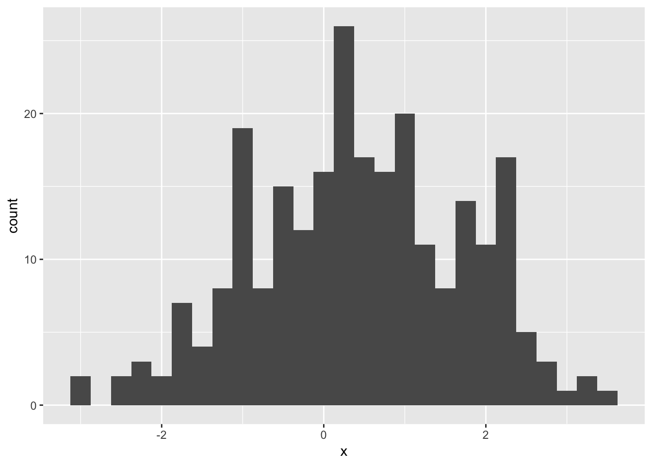
Consider the following sample, \(n = 250\)

ggplot(mapping = aes(x = x)) +
  geom_histogram(binwidth = 0.25)

One model might be a two component Normal mixture: arises when with probability \(\pi\) we get a value from N\((\mu_1, \sigma_1^2)\), and otherwise a sample from N\((\mu_2, \sigma_2^2)\).

\[ f(x; \pi, \mu_1, \mu_2, \sigma_1, \sigma_2) = \pi\phi(x; \mu_1, \sigma_1^2) + (1- \pi)\phi(x; \mu_2, \sigma_2^2) \] where \(\phi(x; \mu, \sigma^2)\) is the density function for a Normal(\(\mu, \sigma^2)\).

Your Turn

Let \(\theta = (\pi, \mu_1, \mu_2, \sigma_1, \sigma_2)\).

Fill in the body of the function to calculate the density function for a specified theta and data vector x:

dmix <- function(x, theta){
  pi <- theta[1]
  mu_1 <- theta[2]
  mu_2 <- theta[3]
  sigma_1 <- theta[4]
  sigma_2 <- theta[5]
  pi * dnorm(x, mean = mu_1, sd = sigma_1) +
   (1 - pi) * dnorm(x, mean = mu_2, sd = sigma_2) 
} 
dmix(0, c(0, 1, 1, 1, 1))

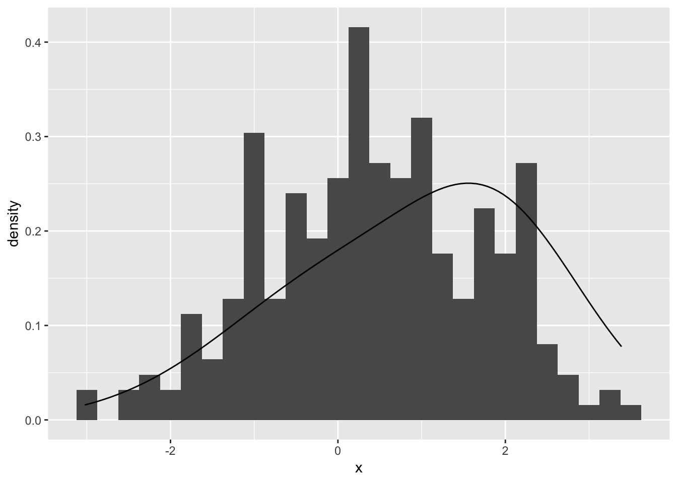
## [1] 0.2419707

Then try some more reasonable parameters to compare to the data:

ggplot(mapping = aes(x = x)) +
  geom_histogram(aes(y = stat(density)), binwidth = 0.25) +
  stat_function(fun = dmix, args = list(theta = c(0.6, 0.2, 2, 1.5, 1)))

Find MLE with maximization

Need negative log likelihood:

nllhood_mix <- function(theta, x){
  d <- dmix(x, theta)
  -1 * sum(log(d))
}

optim() with method = "BFGS", does a Quasi Newton method (swaps Hessian with an approximation).

Your Turn Provide starting values to the par argument: par is like the \(\mathbb{x}_0\) above, values for \(\theta\) we think are close to the values that give the minimum:

Things that go wrong

• Lot’s of messages - bad parameter values lead to messages with NaN
• Non convergence no convergence due to bad parameter values
• Local minima

Lot’s of messages

This converges, $convergence is 0, but we get a lot of messages about NaN. This happens when a call to nllhood_mix() returns NaN, mostly when using bad values for the parameters, e.g. \(\pi = -1\), or \(\sigma_1 < 0\).

(mle1 <- optim(par = c(1, 0, 1.8, 1.2, 0.7), fn = nllhood_mix, x = x, method = "BFGS"))

## $par
## [1] 0.9362468 0.3054438 2.2488241 1.2412696 0.1166007
## 
## $value
## [1] 411.6919
## 
## $counts
## function gradient 
##      125       41 
## 
## $convergence
## [1] 0
## 
## $message
## NULL

optim() can handle this fine, so we don’t really need to worry.

To avoid NaN warnings we could protect our function from returning values at bad parameter values:

nllhood_mix2 <- function(theta, x){
  d <- dmix(x, theta)
  if (any(d < 0) || any(is.nan(d))){
    return(Inf)
  }
  -1 * sum(log(d))
}

But this does introduce some weird discontinuities in our function.

optim(par = c(0.4, 2, -0.2, 1, 2), fn = nllhood_mix2, x = x, 
  method = "BFGS")

## $par
## [1] 0.06375411 2.24883288 0.30540257 0.11662763 1.24126413
## 
## $value
## [1] 411.6919
## 
## $counts
## function gradient 
##       72       19 
## 
## $convergence
## [1] 0
## 
## $message
## NULL

Or use a bounded algorithm (see below).

Non-convergence

This doesn’t converge, $convergence is 1,:

(mle2 <- optim(par = c(0.5, 0, 1, 2, 1), fn = nllhood_mix, x = x, method = "BFGS"))

## $par
## [1] -3410.0610 -6066.8409  -230.4462   550.6597   588.7451
## 
## $value
## [1] -190.2385
## 
## $counts
## function gradient 
##      185      100 
## 
## $convergence
## [1] 1
## 
## $message
## NULL

This means we hit our maximum number of iterations, we can start again from where we finished:

optim(par = mle2$par, fn = nllhood_mix, x = x, method = "BFGS")

## $par
## [1] -3417.3092 -6066.8409  -213.5316   550.6597   551.9619
## 
## $value
## [1] -207.3375
## 
## $counts
## function gradient 
##      100      100 
## 
## $convergence
## [1] 1
## 
## $message
## NULL

But we still don’t converge. In this case, our likelihood rapidly decreases away from the parameter space.

Local minima

These starting parameters converge (with reasonable values of parameters) but not to the global minimum:

(mle3 <- optim(par = c(0.5, 1, 1, 1, 1), fn = nllhood_mix, x = x, method = "BFGS"))

## $par
## [1] 0.5000000 0.4293384 0.4293384 1.2918282 1.2918282
## 
## $value
## [1] 418.7493
## 
## $counts
## function gradient 
##       30       10 
## 
## $convergence
## [1] 0
## 
## $message
## NULL

mle3$par

## [1] 0.5000000 0.4293384 0.4293384 1.2918282 1.2918282

Notice the value of the negative log likelihood, 418.7, is bigger than that at the other minimum 411.7. This is a local minimum.

Always try a few values for the starting parameters.

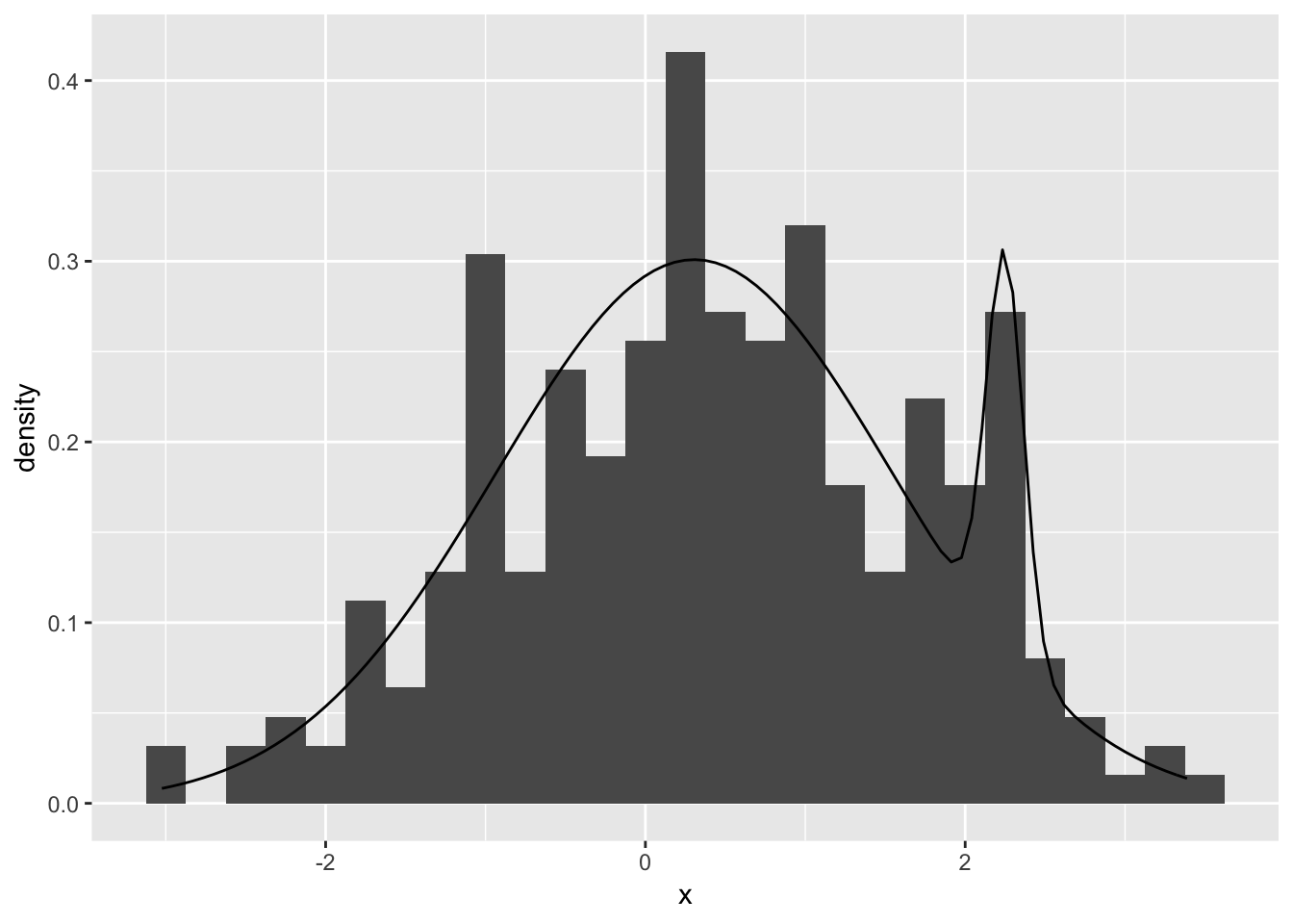
Our MLE fit

ggplot(mapping = aes(x = x)) +
  geom_histogram(aes(y = stat(density)), binwidth = 0.25) +
  stat_function(fun = dmix, args = list(theta = mle1$par))

Derivatives

We didn’t supply the gradient – optim() will numerically approximate it with a finite difference.

Practical issues with general optimzation often have less to do with the optimizer than with how carefully the problem is set up.

In general it is worth supplying a function to calculate derivatives if you can, although it may be quicker in a one-off problem to let the software calculate numerical derivatives.

– Ripley, B. D. “Modern applied statistics with S.” Statistics and Computing, fourth ed. Springer, New York (2002).

You can do it “by hand”, or for some simple functions (include things like dnorm()) get R to do it, see ?deriv.

Scaling

It is worth ensuring the problem is reasonably well scaled, so a unit step in any parameter can have a comparable change in size to the objective, preferably about a unit change at the optimium.

– Ripley, B. D. “Modern applied statistics with S.” Statistics and Computing, fourth ed. Springer, New York (2002).

Your Turn

Using nllhood() experiment with some values of theta, how much does the likelihood change for a unit change in pi? Compare it to a unit change in mu_1.

nllhood_mix(theta = c(0.01, -0.2, 2, 2, 1), x = x)

nllhood_mix(theta = c(0.09, -0.2, 2, 2, 1), x = x)

nllhood_mix(theta = c(0.5, -0.2, 2, 2, 1), x = x)

nllhood_mix(theta = c(0.5, 0.8, 2, 2, 1), x = x)

(It will depend on the values of the other parameters, so try some near the values you would guess from the plot)

You can specify a scaling vector with control = list(parscale = c()), “Optimization is performed on par/parscale”:

optim(par = c(0.6, -0.2, 2, 2, 1), fn = nllhood_mix, x = x, 
  method = "BFGS",
  control = list(parscale = c(5, 1, 1, 1, 1)))

## $par
## [1] 0.984634178 0.408660023 1.771180476 1.290380441 0.006545839
## 
## $value
## [1] 415.3845
## 
## $counts
## function gradient 
##      141       23 
## 
## $convergence
## [1] 0
## 
## $message
## NULL

MLE and the Hessian

If \(\hat{\theta}\) is the MLE for \(\theta\), then for large \(n\), \[ \hat{\theta} \dot{\sim} N(\theta, I(\hat{\theta})^{-1}) \]

where \(I(\hat{\theta})\) is the observed Fisher Information matrix, the negative Hessian of the likelihood evaluated at the MLE.

Or, in other words, the standard errors for the estimates are the square root of the diagonal of the inverse observed Fisher Information.

Since we minimized the negative log likelihood, the Hessian returned by optim() is the observed Fisher information matrix.

(mle <- optim(par = c(0.6, -0.2, 2, 2, 1), fn = nllhood_mix, x = x, method = "BFGS",
  hessian = TRUE))

## $par
## [1] 0.9362459 0.3054026 2.2488329 1.2412641 0.1166276
## 
## $value
## [1] 411.6919
## 
## $counts
## function gradient 
##       71       19 
## 
## $convergence
## [1] 0
## 
## $message
## NULL
## 
## $hessian
##            [,1]        [,2]       [,3]        [,4]      [,5]
## [1,] 2410.73545 -133.168404 -82.539755 -123.036544 532.91237
## [2,] -133.16840  141.886434   0.305168   -9.383503  39.56664
## [3,]  -82.53976    0.305168 433.310427   14.567811  63.21927
## [4,] -123.03654   -9.383503  14.567811  294.759788  37.31136
## [5,]  532.91237   39.566643  63.219273   37.311359 367.84043

mle$hessian %>% solve() %>% diag() %>% sqrt()

## [1] 0.02926314 0.09565745 0.05022398 0.06190159 0.07436482

data.frame(
  est = mle$par, 
  se = mle$hessian %>% solve() %>% diag() %>% sqrt()
)

Bounds on parameters

Use method = "L-BFGS-B" and specify lower and upper.