More complicated simulations
Charlotte Wickham
Oct 9th 2018
knitr::opts_chunk$set(echo = TRUE, results = "hide")
library(tidyverse)
set.seed(181871)
Homework #2
findInterval() and Ross’s statement about efficiency.
Easiest to explore by writing functions:
find_int <- function(n, values, probs){
  cumulative_probs <- cumsum(probs)
  u <- runif(n)
  values[findInterval(u, cumulative_probs) + 1]
}
Check with a somewhat extreme example:
values <- c(  1,    2,    3,    4)
probs <- c(0.05, 0.05, 0.10, 0.80)

find_int(n = 1000, values, probs) %>%
  table()
Ross’s suggestion for efficiency is to order by decreasing probability first, e.g.
ind_order <- order(probs, decreasing = TRUE)
(values_ordered <- values[ind_order])
(probs_ordered <- probs[ind_order])

find_int(n = 1000, values_ordered, probs_ordered) %>%
  table()
Now compare timing:
library(bench)
timing_find_int <- press(
  n = c(100, 1000, 10000),
  mark(
    ordered = find_int(n, values_ordered, probs_ordered),
    raw = find_int(n, values, probs),
    check = FALSE
  )
)
## Running with:
## n## 1 100## 2 1000## 3 10000timing_find_int %>%
ggplot(aes(x = n, y = mean,
color = expression, shape = expression)) +
geom_point() +
labs(x = "Sample size", y = "Time",
title = "Comparing ordering for `findInterval()` implementation") +
scale_x_log10()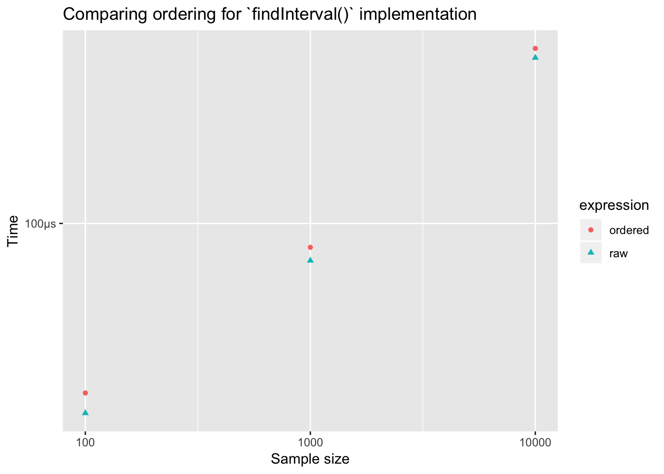
Hardly any difference! Why, findInterval() doesn’t do a sequntial search through the intervals. It does something much more efficient.
Compare to the sequential search:
naive <- function(n, values, probs){
  cumulative_probs <- cumsum(probs)
  u <- runif(n)
  x <- double(n)
  for (i in 1:n){
    if(u[i] < cumulative_probs[1]){
      x[i] <- values[1]
    } else if (u[i] < cumulative_probs[2]){
      x[i] <- values[2]
    } else if (u[i] < cumulative_probs[3]){
      x[i] <- values[3]
    } else {
      x[i] <- values[4]
    }
  }
  x
}
timings <- bench::press(
n = c(100, 1000, 10000),
bench::mark(
findint_ordered = find_int(n, values_ordered, probs_ordered),
findint_raw = find_int(n, values, probs),
naive_ordered = naive(n, values_ordered, probs_ordered),
naive_raw = naive(n, values, probs),
check = FALSE
)
)## Running with:
## n## 1 100## 2 1000## 3 10000timings %>%
ggplot(aes(x = n, y = mean,
color = expression, shape = expression)) +
geom_point() +
labs(x = "Sample size", y = "Time",
title = "Comparing two implementations") +
scale_x_log10()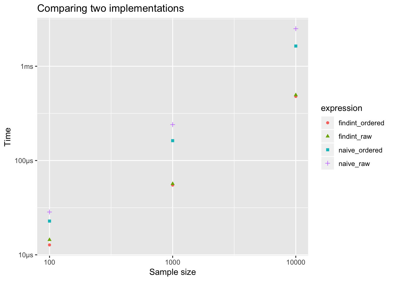
Much bigger difference in a sequential search, but naive sequential search is much slower than findInterval() approach.
Organization
Good enough practices for scientific computing
This paper focuses on these first accessible skills and perspectives – the “good enough” practices for scientific computing: a minimum set of tools and techniques that we believe every researcher can and should consider adopting.
Wilson G, Bryan J, Cranston K, Kitzes J, Nederbragt L, et al. (2017) Good enough practices in scientific computing. PLOS Computational Biology 13(6): e1005510. https://doi.org/10.1371/journal.pcbi.1005510
All the sections are important! We’ll interpret some sections a little differently given our scope.
We’ll return to the article a few times. The project rubric will include following the practices outlined in this article.
Software
The core realization in these practices is that being readable, reusable, and testable are all side effects of writing modular code, i.e., of building programs out of short, single-purpose functions with clearly-defined inputs and outputs. Much has been written on this topic, and this section focuses on practices that best balance ease of use with benefit for you and collaborators.
Place a brief explanatory comment at the start of every program (2a)
Decompose programs into functions (2b)
What’s the difference between a program and a function?
- programs are many functions
- program is complex task -> e.g. simulation study
- program might have mutliple files, function is in a single file.
Rmarkdown often lets us blend the line between program and the documentation of the program. This is good, it encourages us to document as we go.
Sometimes analyses will get complicated enough that a single RMarkdown document isn’t the best way to keep things organized…more on Thursday.
Our old friend the coin toss sequence
A random sequence of H’s and T’s is generated by tossing a fair coin \(n = 20\) times. What’s the expected length of the longest run of consecutive heads or tails?
Taken from Tijms, Henk. Probability: A Lively Introduction. Cambridge University Press, 2017
Some variations
How does the expected length of the longest run vary with the number of coinflips, \(n\)?
How does the answer change if the coin isn’t fair?
How does the expected length of the longest run compare to the median length of the longest run?
How does the variance of our estimate vary with the number of simulations we do?
In each case we are adding an additional parameter to our simulation
How does the expected length of the longest run vary with the number of coinflips, \(n\)?
Your Turn What should our final data look like to construct this plot?
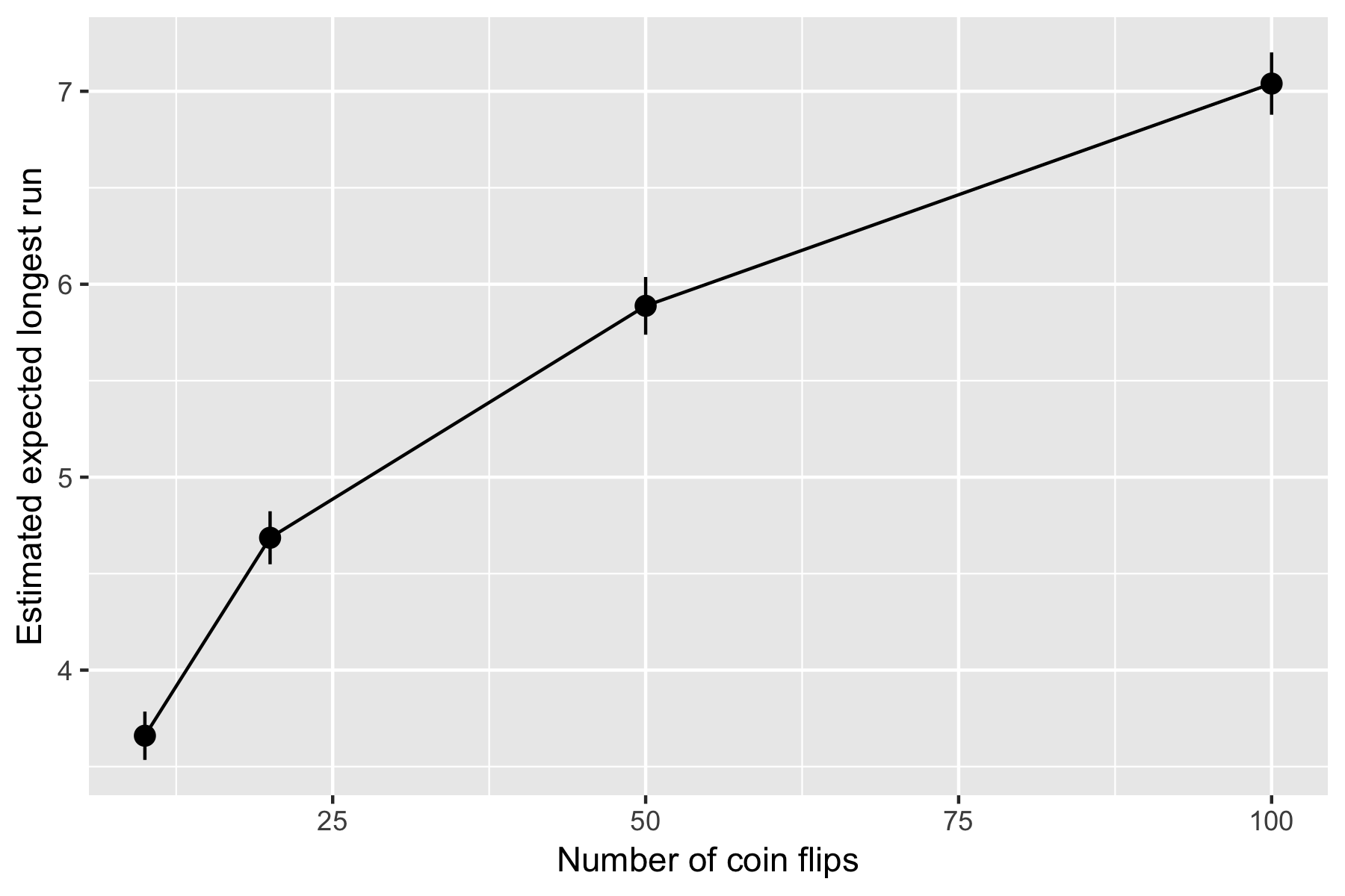
What we want is a 4 row data frame something like this:
n       est     sd
10      ...     ...
20      ...     ...
50      ...     ...
100     ...     ...
New to ggplot, the best place to start is Visualization in R4DS
Setup
A useful break-down of our previous process into a few functions:
sim_coin_tosses <- function(n_sims, n, prob){
  # Simulates n_sims sequences of n coin tosses
  # with heads occuring with probability prob
  # fair, by default
  rerun(n_sims,
    rbinom(n, size = 1, prob = prob))
}

max_run_length <- function(x){
  # Finds length of longest run in x
  max(rle(x)$lengths)
}

sim_run_lengths <- function(n_sims, n, prob = 0.5){
  # Returns length of longest run in n_sims sequences
  # of coin toss sequences of  n flips, where each flip
  # has prob p of being heads.
  sim_coin_tosses(n_sims, n, prob) %>%
    map_dbl(~ max_run_length(.))
}
Your turn What should the output be?
sim_run_lengths(n_sims = 10, n = 4, prob = 1)Now, n the number of flips is an argument to our function.
One approach
How does the expected length of the longest run vary with the number of coinflips, \(n\)?
Set up some values of \(n\)
ns <- c(10, 20, 50, 100)For each element in ns estimate the mean longest run:
Simulate the longest runs for each \(n\):
lengths_for_each_n <- map(ns,
  ~ sim_run_lengths(n_sims = 500, n = .))
Find the mean of each set of longest runs:
map_dbl(lengths_for_each_n, ~ mean(.))
An aside on map() back at 9:03
If the second argument takes the pattern ~ fun(.), you can just supply fun without using the formula notation:
map_dbl(lengths_for_each_n, ~ mean(.))
# is the same as
map_dbl(lengths_for_each_n, mean)
You can supply addtional arguments to map() which will be passed on to the function in the second argument. For example, pass on argument to mean():
map_dbl(lengths_for_each_n, mean, na.rm = TRUE)Or in our example:
lengths_for_each_n <- map(ns,
  ~ sim_run_lengths(n_sims = 500, n = .x))
# is the same as
lengths_for_each_n <- map(ns,
  sim_run_lengths,
  n_sims = 500)
Student question: Can we do more than one thing to an element? Yes, but you end up with more complicated data structures:
map(lengths_for_each_n,
  ~ list(mean(.), sd(.)))
I’d reccomend just doing it twice
map(lengths_for_each_n, mean)
map(lengths_for_each_n, sd)
Key ideas
Storing more complicated simulations in tibbles/data frames let’s you leverage other data manipulation tools (e.g. ggplot2, dplyr)
Now you know
map(), the purrr functionsmap2(),pmap()provide an easy extension for you to iterate over more than one object.
Storing a simulation in a data frame
Our current process:
ns <- c(10, 20, 50, 100)
lengths_for_each_n <- map(ns,
  ~ sim_run_lengths(n_sims = 500, n = .x))
map_dbl(lengths_for_each_n, ~ mean(.x))
But ns, lengths_for_each_n and our results are:
- all the same length,
- have corresponding elements.
Makes sense to keep them all together and lined up.
Join them up afterwards (OK, but better way soon):
sims <- data_frame(
  n = ns,
  n_sims = 500,
  run_lengths = lengths_for_each_n,
  est = map_dbl(lengths_for_each_n, mean)
)
sims
Advantages
Easy manipulation with dplyr:
sims <- sims %>%
  mutate(
    sd = map_dbl(run_lengths, sd)
  )
Easy plotting with ggplot:
sims %>%
  ggplot(aes(n, est)) +
    geom_pointrange(aes(
      ymin = est - 1.96*sd/sqrt(n_sims),
      ymax = est + 1.96*sd/sqrt(n_sims))) +
    geom_line() +
    labs(x = "Number of coin flips", y = "Estimated expected longest run")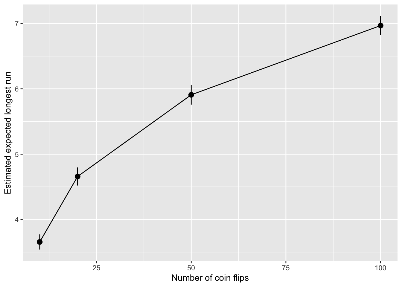
Everything we need is in one object, easy to save for later:
write_rds(sims, "max-run-length-by-n-simulations.rds")write_rds() is a function in readr.
Build it up as we go
A better approach is to start with a data frame from the outset:
sims <- data_frame(
  n = ns
)
Also forces you to think about the parameters of the simulation (i.e. what should vary?)
Now our operations happen within the data frame, dplyr::mutate() adds new columns, here one generated by a map() over the n column:
sims_with_lengths <-
  sims %>%
    mutate(run_lengths = map(n, sim_run_lengths,
      n_sims = 500))
Calls to map_dbl() or map_int() etc, get us columns of numbers:
sims_with_stats <-
  sims_with_lengths %>%
    mutate(
      mean_longest_run = map_dbl(run_lengths, mean),
      sd_longest_run = map_dbl(run_lengths, sd))

sims_with_stats
Iterating over more than one object
Pick up here Thursday
ns
(ps <- seq(0.1, 0.9, by = 0.2))
Now what is the expected length of the longest run for every combination of \(n\) and \(p\)?
(all_ns <- rep(ns, each = length(ps)))
(all_ps <- rep(ps, times = length(ns)))
When you need to iterate over more than one thing map2() and pmap()
Recall, this translates to “for each element of .x, do .f”:
map(.x, .f)map2() extends this when you need to iterate of two objects, “for each element of .x and .y do .f”
map2(.x, .y, .f)But now .f should take two arguments.
A simpler example
map2(.x = c(1, 2, 3), .y = c(-1, 0, 1),
  ~ .x * .y)
Or ask for a simple object with the map2_***() functions, e.g. a double vector:
map2_dbl(.x = c(1, 2, 3), .y = c(-1, 0, 1),
  ~ .x * .y)
In our situation
map2(all_ns, all_ps,
  ~ sim_run_lengths(10, n = .x, prob = .y)) # 10 just as an example
This doesn’t work here, since each element is longer than length 1:
map2_dbl(all_ns, all_ps,
  ~ sim_run_lengths(10, n = .x, prob = .y)) # 10 just as an example
## Error: Result 1 is not a length 1 atomic vectorHard to keep track of which belongs to which…so start with a data frame:
simulation_params <- list(
  n = ns, prob = seq(0.1, 0.9, by = 0.2)
)

runs <- cross_df(simulation_params)
Use dplyr to add columns:
runs <- runs %>%
  mutate(
    run_lengths = map2(.x = n, .y = prob,
      ~ sim_run_lengths(n_sims = 500, n = .x, prob = .y)))

runs <- runs %>%
  mutate(
    mean_max_length = map_dbl(run_lengths, mean),
    sd_max_length = map_dbl(run_lengths, sd),
    n_sims = map_dbl(run_lengths, length)
  )
Easy to plot and manipulate:
runs %>%
  ggplot(aes(x = n, y = mean_max_length, color = factor(prob))) +
    geom_pointrange(aes(
      ymin = mean_max_length - 1.96*sd_max_length/sqrt(n_sims),
      ymax = mean_max_length + 1.96*sd_max_length/sqrt(n_sims))) +
geom_line() 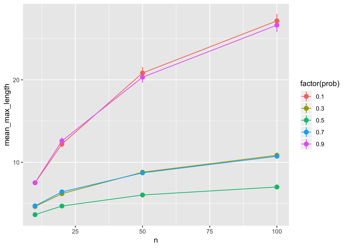
More complicated simulations…
Switching to a dataframe, maybe use pmap():
simulation_params_big <- list(
  n = ns,
  prob = seq(0.1, 0.9, by = 0.2),
  n_sims = c(100, 1000, 10000)
)

runs_big <- cross_df(simulation_params_big)
Use dplyr to add columns:
runs_big <- runs_big %>%
  mutate(
    run_lengths = pmap(list(n = n, prob = prob, n_sims = n_sims),
      sim_run_lengths)) %>%
  mutate(
    mean_max_length = map_dbl(run_lengths, mean),
    sd_max_length = map_dbl(run_lengths, sd)
  )
A data frame is a list, so you could also do:
runs_big <- cross_df(simulation_params_big)
pmap(runs_big,
      sim_run_lengths) %>%
  bind_cols(runs_big)
Easy to plot and manipulate:
runs_big %>%
  ggplot(aes(x = n, y = mean_max_length, color = factor(prob))) +
    geom_pointrange(aes(
      ymin = mean_max_length - 1.96*sd_max_length/sqrt(n_sims),
      ymax = mean_max_length + 1.96*sd_max_length/sqrt(n_sims))) +
    geom_line()  +
  facet_wrap(~ n_sims)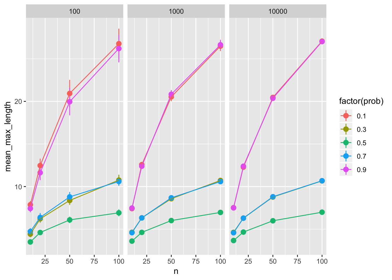
Next time
Project organization, you will work in RStudio Cloud, be prepared.
Back at 8:53am