What about empirical comparisons of variance?

When our parameter of interest can be written as an expectation, we can use the CLT to guide us in quantifying the variance in our estimate.

But sometimes this might not be enough if:

1. We aren’t convinced the CLT has kicked in
2. We aren’t in a situation where the CLT applies (we aren’t using a sample average)

We could use simulation to estimate it…

Simulating to find the variance of a simulation estimate

One estimate of the required expectation:

num_sims <- 1000
many_sequences <- rerun(num_sims, 
  rbinom(20, size = 1, prob = 0.5))
longest_runs <- map_dbl(many_sequences, 
  ~ max(rle(.)$lengths))
mean(longest_runs)

## [1] 4.657

Another…

many_sequences <- rerun(num_sims, 
  rbinom(20, size = 1, prob = 0.5))
longest_runs <- map_dbl(many_sequences, 
  ~ max(rle(.)$lengths))
mean(longest_runs)

## [1] 4.662

But…really we want to automate this.

Take the same approach

1. Simulate: repeat the prior simulation many times, each time getting an estimate of the desired expectation: mean(longest_runs)
2. Calculate: nothing extra to do (flatten_dbl())
3. Summarize: sample variance of estimated expectations

The first step is now simulating a complicated thing, so wrap it up into a function:

mc_estimate_run_length  <- function(num_sims){
  # estimate the expected maximum run of H or T
  # in 20 coin flips by monte carlo
  many_sequences <- rerun(num_sims, 
    rbinom(20, size = 1, prob = 0.5))
  longest_runs <- map_dbl(many_sequences, 
    ~ max(rle(.)$lengths))
  mean(longest_runs)
}
mc_estimate_run_length(1000)

## [1] 4.608

many_estimates <- rerun(500, mc_estimate_run_length(num_sims = 1000))
many_estimates_flat <- many_estimates %>% flatten_dbl() 

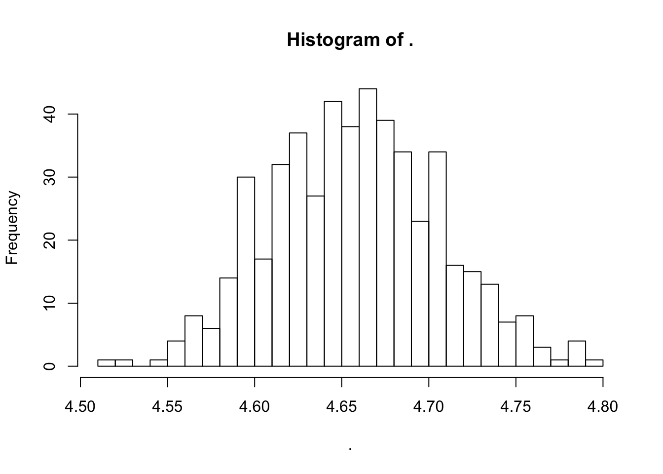
many_estimates_flat %>% hist(breaks = 20)

sd(many_estimates_flat)

## [1] 0.04846478

sd(longest_runs)/sqrt(1000)

## [1] 0.04835384

Compares well to our estimate that relied on the CLT (it should, the CLT should be pretty good for \(n = 1000\))

many_estimates %>% flatten_dbl() %>% sd(na.rm = TRUE) 

## [1] 0.04846478

sd(flatten_dbl(many_estimates), na.rm = TRUE)

## [1] 0.04846478

Your turn

Estimate the standard deviation of our MC based estimate, when we simulate just 250 coin toss sequences in each simulation.

many_estimates <- rerun(500, mc_estimate_run_length(num_sims = 250))
many_estimates_flat <- many_estimates %>% flatten_dbl() 
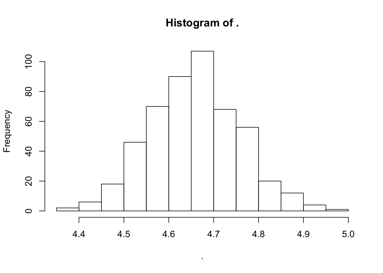
many_estimates_flat %>% hist(breaks = 20)

sd(many_estimates_flat)

## [1] 0.09933127

Does you answer agree with what the CLT might predict?

Back at 8:55am

Careful with \(n\)

Lot’s of sample sizes floating around:

• 500 the number of simulations we use to estimate the variance
• 1000 the number of simulations of coin toss sequences in each estimate of the expectation
• 20 the number of coins flipped

(that’s 10 million coin flips total)

An example

Let \(X \sim\) Uniform(0, 1). What is \(\text{E}\left(e^x\right)\)?

(We could answer this with calculus quite easily…but it’s a nice example to work with)

The naive MC approach:

n_sims <- 500
many_x <- runif(n_sims)
exp_many_x <- exp(many_x)
mean(exp_many_x) # our estimate of E(e^x)

## [1] 1.731394

# rough CI half-width on this estimate
(naive_ci_halfwidth <- 1.96*sd(exp_many_x)/sqrt(n_sims))

## [1] 0.04364225

(Don’t need rerun() here, it’s easy to get many samples from a Uniform)

The antithetic variable approach

\(h(X) = e^x\) is monotone in \(x\).

So, we should be able to reduce variance by generating pairs of negatively correlated draws from a Uniform(0, 1).

One set of pairs: \((X, 1-X)\) where \(X \sim\) Uniform(0, 1)

Both \(X\) and \(1-X\) have the right distribution and are negatively correlated.

x_first_in_pair <- runif(n_sims/2) # need half as many draws
x_second_in_pair <- 1 - x_first_in_pair

# a useful function in this example
pair_average <- function(x1, x2){
  1/2 * (x1 + x2)
}

pair_averages <- pair_average(x1 = exp(x_first_in_pair), 
  x2 = exp(x_second_in_pair))

mean(pair_averages) # our estimate of E(e^x)

## [1] 1.719627

# rough CI half-width on this estimate
(antithetic_ci_half_width <- 1.96*sd(pair_averages)/sqrt(n_sims/2))

## [1] 0.008172898

5 times smaller!

Antithetic variables takeaways

• Need to be in a setting where the \(\text{E}(h(X))\) is of interest
• \(h(x)\) needs to be monotone
• Can get big variance reductions
• You might only need to sample half as many points