Warm up…the challenge from last time

A random sequence of H’s and T’s is generated by tossing a fair coin \(n = 20\) times. What’s the expected length of the longest run of consecutive heads or tails?

Taken from Tijms, Henk. Probability: A Lively Introduction. Cambridge University Press, 2017.

My take

Out of 30 submissions, 7 unique articles that had some substantial computation, in three broad categories:

• Simulation of a complex (or simple) process, and summaries of the resulting distributions
  • F. Din-Houn Lau and Axel Gandy [2016] Enhancing football league tables. https://rss.onlinelibrary.wiley.com/doi/epdf/10.1111/j.1740-9713.2016.00956.x
  • A variation of the birthday problem - a reader responds, Friedman, E.M., https://www.significancemagazine.com/science/422-a-variation-of-the-birthday-problem-a-reader-responds
  • How our election forecast model at the Polling Observatory works, Robert Ford, Will Jennings, Mark Pickup & Christopher Wlezien https://www.significancemagazine.com/politics/272-how-our-model-at-the-polling-observatory-works
• A analysis of a single dataset using a computationally intensive tool
  • Meyer, Renate, and Nelson Christensen. “Gravitational waves: A statistical autopsy of a black hole merger.” Significance 13.2 (2016): 20-25. https://doi.org/10.1111/j.1740-9713.2016.00896.x
  • Paulden, T. (2016), Smashing the racket. Significance, 13: 16-21. doi:10.1111/j.1740-9713.2016.00914.x
• A comparison of many statistical methods over simulated datasets
  • Citation: Eklund, A. and Nichols, T. (2017), How open science revealed false positives in brain imaging. Significance, 14: 30-33. doi:10.1111/j.1740-9713.2017.01000.x

Articles providing enough links to code and data to reproduce the analysis were rare.

Project

Proposals will be due as part of homework #3. (More details on what a proposal looks like then).

Start thinking about what you’d like to work on.

It probably will fit into one of the three categories above, or additionally you might aim to implement a statistical algorithm of interest.

It should stretch your current abilities.

I would expect over the quarter you put in ~ 40 hours. (planning, implementation (coding), making the implementation nice, documentation, communication).

I’m here to help, with some indication of your interests.

One pretty flexible approach

1. Simulate many examples (rerun())
2. Calculate something on each example (map(), map_dbl())
3. Explore the many calculated things (# depends on goal)

The challenge from last time

A random sequence of H’s and T’s is generated by tossing a fair coin \(n = 20\) times. What’s the expected length of the longest run of consecutive heads or tails?

Taken from Tijms, Henk. Probability: A Lively Introduction. Cambridge University Press, 2017.

# A single simulated example 1 = H, 0 = T
one_sequence <- rbinom(20, size = 1, prob = 0.5)

# Longest run?
max(rle(one_sequence)$lengths)

## [1] 5

All together…

num_sims <- 1000
many_sequences <- rerun(num_sims, 
  rbinom(20, size = 1, prob = 0.5))
longest_runs <- map_dbl(many_sequences, 
  ~ max(rle(.)$lengths))

# Finally...
mean(longest_runs)

## [1] 4.639

Ways things get more complicated

1. The thing you are simulating is complicated.
2. The thing you are calculating is complicated.
3. The thing you are simulating or calculating depends on some parameters and you want to explore how they affect the result.

Solve 1. and 2. by writing functions, 3. with further iteration.

Functions - Your Turn

(4 min)

• What are the three key steps to writing a function? Assuming you already have a working snippet of code

  1. Choose a good name - really important!!
  2. Define the arguments
  3. Write the body

• Turning the following snippet into a function:

x <- 1:10

# sd_over_mean
# ratio_function
# cv

# a minimal version
coefficient_of_variation <- function(x){
  sd(x, na.rm = TRUE) / mean(x, na.rm = TRUE)
}

# our final version
coefficient_of_variation <- function(x, na.rm = FALSE, ...){
  sd(x, na.rm = na.rm) / mean(x, na.rm = na.rm, ...)
}

x <- runif(10)
coefficient_of_variation(x = x)

## [1] 0.4623089

coefficient_of_variation(x = x, trim = 0.25)

## [1] 0.4564815

Exponential Inverse Transform

From last week: to generate a sample from Exp(\(\lambda\))

u <- runif(1)
lambda <- 5
(x <- -1 / lambda * log(1 - u))

## [1] 0.1018719

Your turn Turn this into a function. What should the arguments be?

u <- runif(1)
lambda <- 5
(x <- -1 / lambda * log(1 - u))

## [1] 0.02019427

sample_exp <- function(n, lambda){
  u <- runif(n)
  -1 / lambda * log(1 - u)
}

sample_exp(10, lambda = 5)

##  [1] 0.1519967204 0.1512896536 0.0042851299 0.1562532665 0.2497672581
##  [6] 0.1366965437 0.2555457133 0.0002328799 0.1706922360 0.0479803846

Back at 9:03

Inverse Transform

What if we wanted this to work for any inverse CDF function?

exp_icdf <- function(u, lambda) {-1 / lambda * log(1 - u)}

u <- runif(1)
exp_icdf(u, lambda = 5)

## [1] 0.1628068

sample_inverse_cdf <- function(n, inv_cdf, ...){
  u <- runif(n)
  inv_cdf(u, ...)
}
sample_inverse_cdf(20, exp_icdf, lambda = 5)

##  [1] 0.053899622 0.025974188 0.165090472 0.711054570 0.313451911
##  [6] 0.257789633 0.103208275 0.184061036 0.175007737 1.020635893
## [11] 0.122751554 0.280594812 0.412539486 0.016316951 0.012855245
## [16] 0.046939276 0.071643537 0.157593954 0.007222465 0.207302211

Your Turn Try it to simulate 100 values from a Normal(0, 1). Hint: you can use the built-in inverse CDF function qnorm().

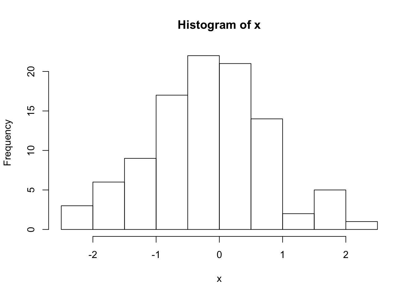
qnorm(0.5) # can use the built in quantile function 

## [1] 0

x <- sample_inverse_cdf(100, qnorm) 
hist(x) # Looks good

# The `...` allow us to pass in other parameters to our inverse 
# CDF function
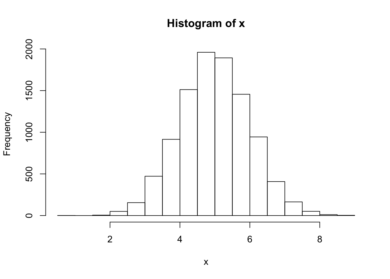
x <- sample_inverse_cdf(10000, qnorm, mean = 5) 
hist(x) # Now centered at 5

Takeaways

• Use functions to remove duplication and wrap-up important pieces of code
• You can pass functions into other functions in R (super useful technique we will see over and over again)

(Pick up here on Thursday)

How big a simulation should we run?

How accurately do we want to estimate \(\theta\)?

Your Turn Can you get a confidence interval on the estimate of the expected length of the longest run from our earlier example?

theta_hat <- mean(longest_runs)

# 95%
theta_hat + c(-1, 1) * 1.96 * (sd(longest_runs)/sqrt(num_sims))

## [1] 4.542639 4.735361

CLT

Let \(Y = h(X)\), \(\mu = E(Y)\) and \(\overline{Y} = \sum_{i = 1}^n h(X_i)\).

Then \[ \text{Var}(\hat{\theta}) = \text{Var}(\overline{Y}) \dot \sim \, N\left(\mu, \frac{\text{Var}(Y)}{n}\right) \] for large \(n\) by the Central Limit Theorem.

We don’t know \(\text{Var}(Y)\), but we can estimate it using our simulated \(Y_i\).

Leads to the usual 95% CI formula: \[ \overline{Y} \pm 1.96 \frac{s}{\sqrt{n}} \] where \(s\) is the sample standard deviation of the \(Y_i\), and \(n\) the number of simulations.

A special case: binary outcomes

New question: What’s the probability of a run greater than 10?

Want to know: \[ p = \text{P}(h(\pmb{X}) = 1) \] where \[ h(\pmb{X}) = \begin{cases} 1, \, \text{when longest run in sequence } \pmb{X} \text{ is greater than 10}, \\ 0, \, \text{otherwise} \end{cases} \] same as asking for \(p =\theta = \text{E}\left( h(\pmb{X})\right)\).

We already have enough to get this new function of our samples:

longest_runs > 10

Estimate \(\theta\) with:

p_hat <- mean(longest_runs > 10)

What’s \(Var(\hat{\theta})\) in this setting?

Use result from Bernoulli random variables \[ Var(\hat{p}) = p(1 - p) \]

Leads to a CI based only on the estimated probability:

p_hat + c(-1, 1) * 1.96 * (sqrt(p_hat*(1-p_hat))/sqrt(num_sims))

## [1] 0.0006282772 0.0093717228

The mean approach still works, but will give slightly different values:

p_hat + c(-1, 1) * 1.96 * (sd(longest_runs > 10)/sqrt(num_sims))

## [1] 0.0006260897 0.0093739103

How big a simulation?

• Base it on a desired width of CI (you might need a pilot simulation to estimate the variance first)
• Simulate again and decide if the next estimate is “close enough” to the first (if not, increase the simulation size)

Next time

Simulating in clever ways to reduce the variance of the estimate, \(\text{Var}(\hat{\theta})\).